- make_db.R - load data into SQLite
- predict.R - make predictions (except for Stan model)
- sparse_glm_csr.stan - Stan model code
- stan.R - make input for Stan model, read results and make final prediction
This is a description of my Melbourne Datathon 2017 Kaggle entry, which came third. See also: Yuan Li's winning entry.
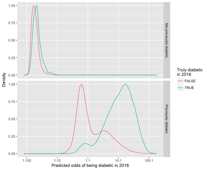
The data this year was drug purchases at pharmacies from 2011-2015. The objective was then to maximize the ROC AUC when predicting the probability of a person purchasing diabetes medication in 2016.
This entry spent quite a lot of time at the top of the leaderboard, however this was merely because the experienced Kaggle players only submitted in the last couple of days. On the plus side, I guess this gave new players a chance to compete with each other rather than be faced with a seemlingly insurmountable AUC from the start.
One thing I wondered was how much I should discuss my entry with other people or keep it secret. Well it was much more fun when I chatted than when I keept silent, and I needn't have worried anyway. The whole thing was a great learning exercise, I've learned some things sure to be relevant to my own work.
Features
All models I used followed a pattern of predicting the binary outcome for each patient (diabetes medication purchased in 2016) from a collection of predictor variables. These predictors were stored in a large, sparse matrix.
I actually used two predictor matrices, one for logistic regression prediction, and a larger one for tree prediction with XGBoost. XGBoost seems able to handle a very large number of predictor variables.
The logistic regression predictors were:
- Purchased a diabetes drug prior to 2016.
- Year of birth, missing values set to 1921.
- Year of birth, missing values set to 2016.
- Known to be female.
- Known to be male.
- Patient location code.
- For each drug, number of purchases, transformed log(1+x).
- For each drug, number of purchases in 2015, transformed log(1+x).
- For each chronic illness, number of drug purchases, transformed log(1+x).
- For each chronic illness, number of drug purchases in 2015, transformed log(1+x).
- For each prescriber, 1 if had a prescription from prescriber else 0.
- For each store, proportion of purchases from store (ie rows normalized to sum to 1).
log(1+x) transformation worked better than either using the count as-is or an indivator variable of whether the count was non-zero. I view it as an intermediate between these extremes.
Additionally the XGBoost predictor matrix contained number of drug purchases in the second half of 2015, from 2014, from 2013, and from 2012.
All features were standardized to have standard deviation one.
Principal Component augmentation
I used the R package irlba to augment the feature matrices with their principal components. Irlba is able to perform SVD on large sparse matrices.
I added 10 principal component columns to the matrix for tree models, and 20 to the matrix for logistic regression models. The main limitation here was that irlba started breaking or running a very long time when asked for more than this.
One interesting thing here is that this adds an aspect of unsupervised learning that includes the test-set patients.
Bootstrap aggregation ("bagging")
I wanted to take model uncertainty into account. If one possible model makes a very strong prediction, and another makes a weaker prediction, I wanted an intermediate prediction. The most likely model might not well characterize the full spread of possibilities.
To this end, each model was bootstrapped 60 times. Probabilities from these 60 bootstraps were averaged. The idea here is to obtain marginal probabilities, integrating over the posterior distribution of models. (Someone more familiar with the theory of bootstrapping could maybe tell me if this is a correct use of it. It certainly improved my AUC.)
Boostrapping is based on sampling with replacement. My bootstrapper function had one slightly fancy feature: overall, each data point is used the same number of times. Within this constraint, it mimics the distribution produced by sampling with replacement as closely as possible. I call this a "balanced bootstrap".
Since bootstraps always leave out about a third of the data, averaging over predictions from the left-out data provides a way to get probabilities for training-set patients that are not over-fitted. These are then used when blending different models. My "balanced bootstrap" scheme ensured every training-set patient was left out of the same proportion of bootrstaps, and I could dial the whole thing down to 2 bootstraps and still have it work if I wanted.
Blending models
The probabilities produced by different models were linearly blended so as to maximize AUC. I again used my bootstrapper to perform this, so I had a good prediction of how accurate it would be without needing to make a Kaggle submission. (Once you have a hammer...)
On to the models themselves.
Regularized logistic regression with glmnet
glmnet fits generalized linear models with a mixture of L2 (ridge) and L1 (lasso) regularization. I used glmnet to perform logistic regression.
glmnet's alpha parameter determines the mixture of L2 and L1 regression. alpha=0 means entirely L2 and alpha=1 means entirely L1. I found a tiny bit of L1 improved predictions slightly over purely L2 regularization. In the end I made one set of predictions using alpha=0.01 and one with alpha=0.
A neat feature of glmnet is that it fits a range of regularization amounts (lambda parameter) in one go, producing a path through coefficient space. As described above, I am always fitting models to bootstrapped data sets. I choose an optimal value for lambda each time to maximize the AUC for the patients left out by the bootstrap.
I want to mention one of the strengths of glmnet but not so relevant to a Kaggle competition: if you turn up alpha close or equal to 1, and turn up lambda high enough, it will produce a sparse set of coefficients with few enough non-zero coefficients that the model is interpretable. Here I've used a low value of alpha to get as accurate predictions as possible, but if I wanted an interpretable model I would do the opposite.
Gradient boosted decision trees with XGBoost
Speaking of non-interpretable models, my next and individually most accurate set of predictions came from XGBoost.
XGBoost creates a stack of decision trees, each tree additively refining the predicted log odds ratio for each patient. By piling up trees like this, and rather like glmnet, we have a path from high regularization to low regularization. Again I used the patients left out of the bootstrap sample to decide at what point along this path to stop.
I used a learning rate of eta=0.1, and allowed a maximum tree depth of 12. XGBoost also has lambda and alpha parameters controlling L1 and L2 regularization. However the meaning of these parameters is different to glmnet: lambda is L2 regularization and alpha is L1 regularization. I'm not sure of the units here. I made two sets of predictions, one with lambda=50, alpha=10, and one with lambda=0, alpha=40. L1 regularization can stop to tree splitting before the maximum depth of 12 is reached (I think).
Limiting the learning rate and number of trees also constitutes a form of regularization, even without these explicit regularization parameters. I'm not 100% clear on how all these parameters interact.
Split glmnet
The most important predictor of buying diabetes drugs in 2016 was buying diabetes drugs prior to 2016. I split the data into two parts on this basis, and fitted glmnet models to each.
XGBoost on top of glmnet
I tried running XGBoost starting from half the log odds ratio predicted by glmnet, as an attempt to blend these two approaches more intimately.
Logistic regression with t distribution priors on coefficients with Stan
Stan is a language for writing Bayesian models. A Stan model can then be compiled to a C++ program that performs Hamiltonian Monte Carlo sampling.
This was a late addition. I didn't bootstrap this because it does its own sampling from the posterior, just blended it in 10%-90% with the blend of the predictions described above.
L2 regulatization can be viewed as a prior belief that coefficients have a normal distribution, and L1 regularization can be viewed as a prior belief that coefficients have a Laplace distribution. However my favourite distribution is Student's t distribution, so I wanted to try this as well. The t distribution looks like a normal distribution, but with fat tails. The Laplace distribution has fatter tails than the normal distribution, but the t distribution's fat tails are fatter still.
I constructed a very simple Stan model for logistic regression with t distributed coefficients. To my surprise this worked, and once I figured out how to use the sparse matrix multiplication function it ran within a bearable time. I ran-in the sampler over 100 iterations, then sampled 100 models from the posterior distribution and averaged the predicted probabilities from these models.
I was impressed by Stan, and if I were doing this exercise over would have spent more time on it.
So there you go, that's my Melbourne Datathon 2017 Kaggle entry in all it's horror glory.
Post-competition notes:
I came third on the final leaderboard.
Yuan Li has described their winning solution, which is xgboost based with much better feature engineering than I've used.
The competition allowed me to submit two final entries, and I submitted one with the Stan model contribution and one without. The one without turned out to be the best of the two, by a hair.
A small attempt at interpretable modelling of the data, using L1 regularized logistic regression.
Better at predicting cesation of diabetes medication than starting it: