Consider the problem of finding differentially expressed genes from RNA-seq data.
Review FDR adjusted p-values
Travel to a parallel universe of FDR adjusted confidence bounds
Confident effect sizes for interactions

2017-11-08
Consider the problem of finding differentially expressed genes from RNA-seq data.
Review FDR adjusted p-values
Travel to a parallel universe of FDR adjusted confidence bounds
Confident effect sizes for interactions
A procedure that will reject a null hypothesis only with small probability \(\alpha\).
eg "This gene's expression has log fold change \(e\)."
Binary outcome: reject or do not reject.
Ways to give the reader more freedom:
Only fix \(e\), usually \(e=0\). Tell the reader a \(p\)-value. The reader may choose their desired \(\alpha\), and rejects the null hypothesis if \(p \leq \alpha\).
Only fix \(\alpha\), usually \(\alpha=0.05\). Try all possible \(e\) and tell the reader the set non-rejected values, which form a Confidence Interval or a Confidence Bound.
(Benjamini and Hochberg, 1995)
For a False Discovery Rate of \(q\), given \(p\)-values \(p_1\)…\(p_n\), find the largest set \(S\):
\[ S = \left\{ i : p_i \leq {|S| \over n} q \right\} \]
Snowballing: The more discoveries you make, the lower the threshold for discovery.
No adjustment for multiple testing
False Discovery Rate control
Family-Wise Error Rate control
Allow the reader to choose FDR.
The set of genes with adjusted \(p\)-value \(\leq q\) controls FDR to be \(q\).
Presentation as a "top table": If genes are sorted by \(p\)-value, whatever \(q\) is chosen the set will always be the head of the table.
Snowballing: May end up with a run of equal adjusted \(p\)-values, even if input \(p\)-values are distinct. These genes should be included or excluded as a unit.
Greater correction at top of table: The \(i\)th row in the table has adjusted \(p\)-value \({ n \over i } p_i\) (unless a snowball occurred).
Further filtering of set, eg by fold change, may lose FDR property.
p.adjust(c(0.05, 0.15, 0.3, 0.5), method="BH")
## [1] 0.2 0.3 0.4 0.5
p.adjust(c(0.2, 0.25, 0.3, 0.5), method="BH")
## [1] 0.4 0.4 0.4 0.5
Weak null hypothesis: that the log fold change is non-zero is not saying much. Is the fold change biologically significant?
What to do if we make too many discoveries? Temptation to set a ridiculously small FDR.
Really want to know which are the largest log fold changes.
(McCarthy and Smyth, 2009)
"t-tests relative to a threshold"
A stronger null hypothesis:
Specify \(e\) to be a biologically significant amount.
Table with adjusted \(p\)-values allows reader to choose FDR.
Better but still some problems:
Specify the desired FDR.
Present results as a "top table" that allows the reader to choose \(e\).
If there are too many discoveries, easily choose a larger \(e\) to concentrate on larger effect sizes.

Let \(S(e)\) be the set of genes selected by TREAT, at some fixed FDR (eg 0.05).
These sets nest: if \(e_1 > e_2\) then \(S(e_1) \subseteq S(e_2)\).
Finding \(S(e)\) for a range of \(e\) values leads to a natural ranking. Again we can present results in a "top table".
(Remaining ambiguity in ranking of genes is resolved by \(p\)-values of first set they are not a member of.)
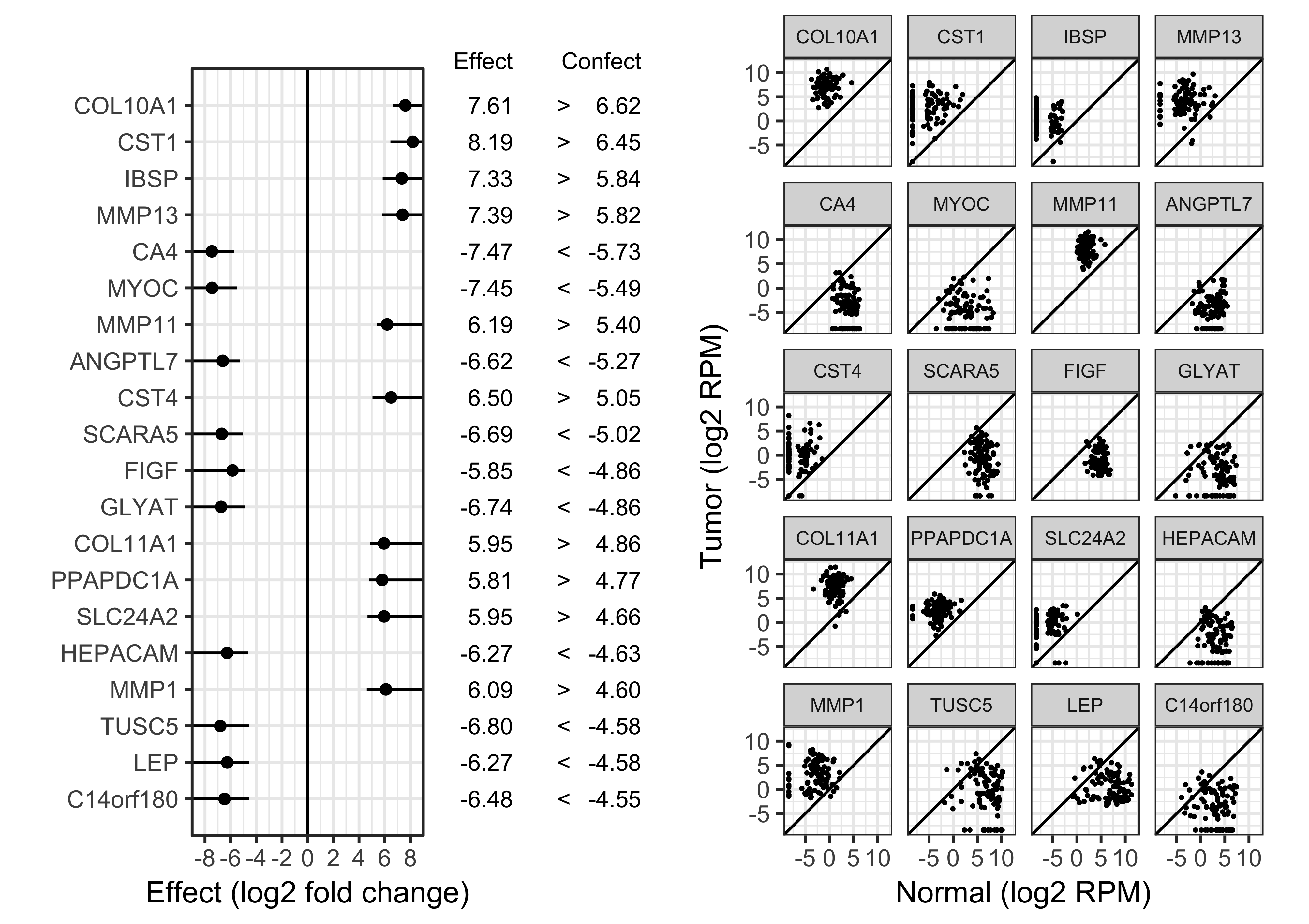
Call the largest \(e\) for which a gene is a member of \(S(e)\) the "confect" (confident effect size) of that gene, with appropriate sign.
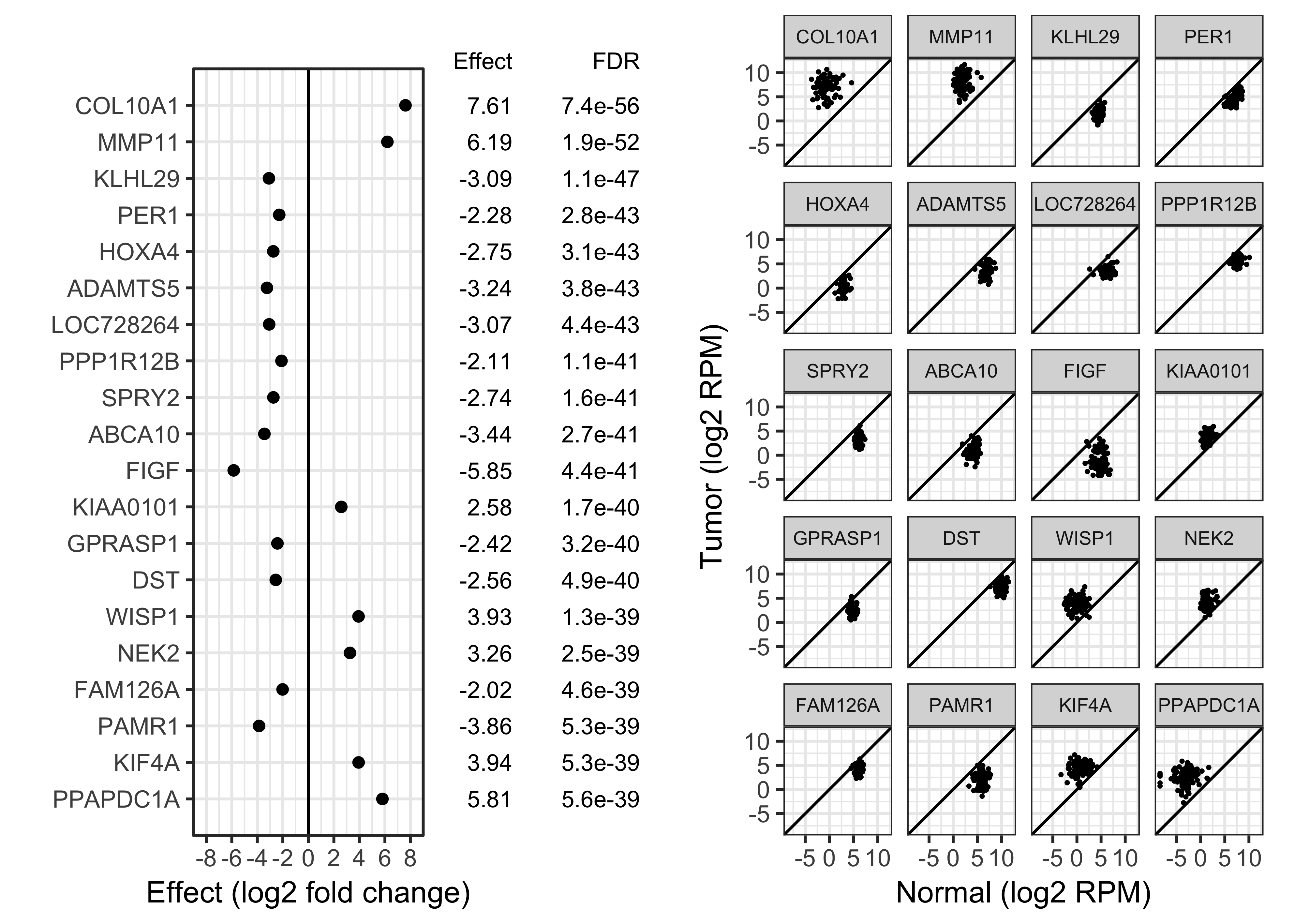
 97 RNA-seq tumor-normal pairs from TCGA.
Shown here, a random sample of 20 genes.
Highly heteroscedastic.
13,416 DE genes at FDR 0.05.
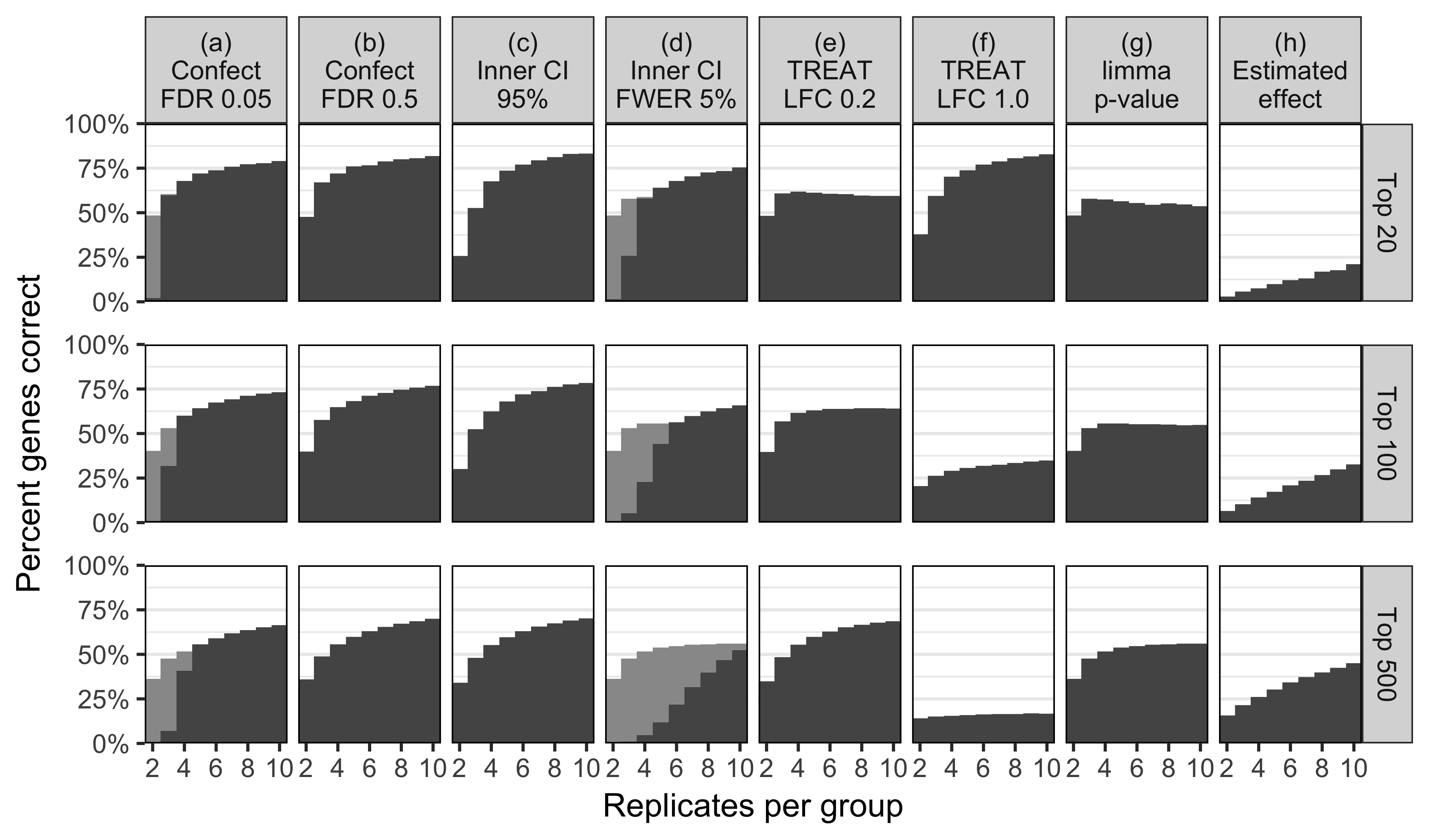
Simulate 15,000 genes \(i\)
\(\mu_{i,2} - \mu_{i,1} \sim 0.15 t(3)\)
\(\sigma^2_i \sim 0.02/{\chi^2_2}\)
(severely heteroscedastic)
Potentially useful for:
Same as \(p\)-value ranking for:
Conventionally, we look for interactions of two experimental factors as a "ratio of ratios". This can be done with linear modelling of log expression levels.
Consider the interaction of two experimental factors A and B.
    B1  B2               B1  B2
A1  20  10           A1  29   1
A2  10  20           A2  26   4

(20/10)/(10/20)      (4/26)/(1/29)
= 4                  = 4.46
Similar effect size, but first case is arguably more interesting.
Consider instead a "difference of proportions".
    B1  B2               B1  B2
A1  20  10           A1  29   1
A2  10  20           A2  26   4

 20/(10+20)              4/(26+4)
-10/(20+10)             -1/(29+1)
= 0.333                 = 0.1
Better represents our interest level.
(Asymmetry between factors may need some care.)
The difference in proportions is 0 in exactly the same cases log(ratio of ratios) is 0.
If we just look for "significance", we see no need to distinguish these two effect sizes, and we may make significant but uninteresting discoveries.
Need to care about magnitude of effect.
GSE80512
Response of wildtype and mutant yeast to high salt concentration.
The mutant has a mutated histone in which post-translational phosphorylation at a certain site is prevented (thought to affect gene regulation).
##         GENENAME     logFC    logCPM        F       PValue          FDR
## YBR021W     FUR4  1.822642  6.299541 224.8724 1.076038e-11 6.224881e-08
## YGR043C     NQM1 -1.465859  9.097715 172.7814 9.774167e-11 2.827178e-07
## YHR096C     HXT5 -1.818737 10.228356 149.9831 3.130767e-10 6.037162e-07
## YJL033W     HCA4  1.491774  4.607822 134.9086 7.402521e-10 9.885850e-07
## YBR072W    HSP26 -1.499280 11.969615 132.5314 8.544382e-10 9.885850e-07
## YOL124C    TRM11  1.271785  4.230186 124.3371 1.426553e-09 1.375434e-06
## YDR070C    FMP16 -1.280466  8.014308 117.7001 2.209317e-09 1.730566e-06
## YHR065C     RRP3  1.185455  4.371145 115.7508 2.522508e-09 1.730566e-06
## YMR011W     HXT2  1.524570 10.194933 114.8032 2.692324e-09 1.730566e-06
## YMR169C     ALD3 -1.054112 11.253244 111.5375 3.382360e-09 1.871477e-06

Note: plots are not log scaled.
## $table
##  rank index confect effect     logCPM    name      GENENAME
##   1    850   0.18    0.2927730  6.299541 YBR021W   FUR4
##   2   5477   0.12    0.2525727 10.194933 YMR011W   HXT2
##   3    469   0.10    0.2196894  5.619169 YJL116C   NCA3
##   4   1692   0.08    0.1715141  9.611573 YDR345C   HXT3
##   5   5208   0.07    0.1596600  8.429903 YHR092C   HXT4
##   6    884  -0.07   -0.2036980  4.193461 YBR056W-A <NA>
##   7   3516   0.07    0.1677288  4.068022 YGR067C   <NA>
##   8   3224   0.06    0.1456658  9.384778 YGL255W   ZRT1
##   9   3735   0.05    0.1208114  3.753062 YLL061W   MMP1
##  10   1888   0.05    0.1455426  8.997924 YIL162W   SUC2
## ...
## 529 of 5785 non-zero effect size at FDR 0.05
## Prior df 6.2
## Dispersion 0.0069 to 0.021
## Biological CV 8.3% to 14.7%

PAT-seq produces reads at 3' ends of transcripts.
Our two interacting factors are:
(((In the talk I demonstrated this with some unpublished data, so I'm not putting it up on the web.)))
https://github.com/pfh/topconfects
devtools::install_github("pfh/topconfects")
library(dplyr)
library(edgeR)
library(limma)
fit <- DGEList(counts) %>%
    calcNormFactors() %>%
    voom() %>%
    lmFit(design)


library(topconfects)
confects <- limma_confects(fit, coef=test_coef, fdr=0.05)
Demonstrated a simple twist on the TREAT method.
Traude Beilharz
Andrew Pattison
David Powell
The results shown here are in whole or part based upon data generated by the TCGA Research Network: http://cancergenome.nih.gov/